Light-cone construction

import numpy as np
import matplotlib.pyplot as plt
from tqdm import tqdm

import tools21cm as t2c

import warnings
warnings.filterwarnings("ignore")

Here we create a fake dataset of coeval cubes which consist of three growing spherical HII regions. The radius is defined using the following form:

\[r = 20~e^{-(z-7)/3}\]

zs_set = np.arange(7,12.1,0.2)

r_hii = lambda x: 30*np.exp(-(x-7.)/3)
plt.plot(zs_set, r_hii(zs_set))

[<matplotlib.lines.Line2D at 0x7fb6143ee110>]

def fake_simulator(ncells, z):
    cube = np.zeros((ncells,ncells,ncells))
    xx, yy, zz = np.meshgrid(np.arange(ncells), np.arange(ncells), np.arange(ncells), sparse=True)
    # rr2 = xx**2+yy**2+zz**2
    r  = r_hii(z)
    r2 = (xx-ncells/2)**2+(yy-ncells/2)**2+(zz-ncells/2)**2
    xx0, yy0, zz0 = int(ncells/2), int(ncells/2), int(ncells/2)
    cube0 = np.zeros((ncells,ncells,ncells))
    cube0[r2<=r**2] = 1
    cube0 = np.roll(np.roll(np.roll(cube0, -xx0, axis=0), -yy0, axis=1), -zz0, axis=2)
    # Bubble 1
    xx1, yy1, zz1 = int(ncells/2), int(ncells/2), int(ncells/2)
    cube = cube+np.roll(np.roll(np.roll(cube0, xx1, axis=0), yy1, axis=1), zz1, axis=2)
    # Bubble 2
    xx2, yy2, zz2 = int(ncells/2), int(ncells/4), int(ncells/16)
    cube = cube+np.roll(np.roll(np.roll(cube0, xx2, axis=0), yy2, axis=1), zz2, axis=2)
    # Bubble 3
    xx3, yy3, zz3 = int(ncells/2+10), int(-ncells/4), int(-ncells/32)
    cube = cube+np.roll(np.roll(np.roll(cube0, xx3, axis=0), yy3, axis=1), zz3, axis=2)
    return cube

Visualizing the fake coeval cubes of growing HII regions.

z0 = 9; c0 = fake_simulator(200,z0)
z1 = 8; c1 = fake_simulator(200,z1)
z2 = 7; c2 = fake_simulator(200,z2)

fig, axs = plt.subplots(1,3, figsize=(14, 5))
axs[0].imshow(c0[100,:,:], origin='lower', cmap='jet')
axs[0].set_title('z={}'.format(z0))
axs[1].imshow(c1[100,:,:], origin='lower', cmap='jet')
axs[1].set_title('z={}'.format(z1))
axs[2].imshow(c2[100,:,:], origin='lower', cmap='jet')
axs[2].set_title('z={}'.format(z2))

Text(0.5, 1.0, 'z=7')

zs_set = np.arange(7,12.1,0.2)
coeval_set = {}
for zi in tqdm(zs_set):
    coeval_set['{:.2f}'.format(zi)] = fake_simulator(200,zi)

100%|██████████| 26/26 [00:07<00:00,  3.29it/s]

Preparing for light-cone construction

To construct light-cones, one can use the make_lightcone function. The parameter filenames takes a list such that each element from this list can be provided to the reading_function to retrieve the coeval cubes for the corresponding redshift (specified in a list by the parameter file_redshifts).

def reading_function(name):
    return coeval_set[name]

filenames = ['{:.2f}'.format(zi) for zi in zs_set]
file_redshifts = zs_set

xf_lc, zs_lc = t2c.make_lightcone(
                            filenames,
                            z_low=None,
                            z_high=None,
                            file_redshifts=file_redshifts,
                            cbin_bits=32,
                            cbin_order='c',
                            los_axis=2,
                            raw_density=False,
                            interpolation='linear',
                            reading_function=reading_function,
                            box_length_mpc=200,
                        )

Making lightcone between 7.000000 < z < 11.999359

100%|██████████| 1256/1256 [00:02<00:00, 605.08it/s]

...done

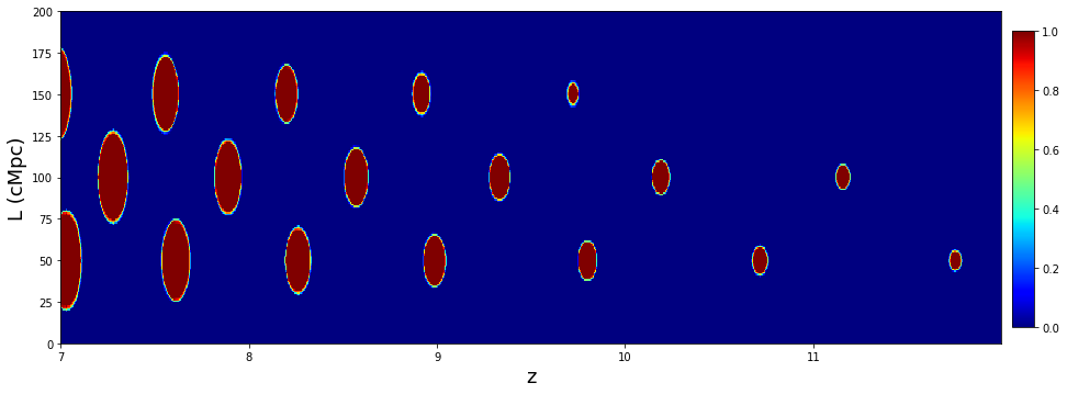
Visualizing the constructed light-cone.

xi = np.array([zs_lc for i in range(xf_lc.shape[1])])
yi = np.array([np.linspace(0,200,xf_lc.shape[1]) for i in range(xi.shape[1])]).T
zj = (xf_lc[100,1:,1:]+xf_lc[100,1:,:-1]+xf_lc[100,:-1,1:]+xf_lc[100,:-1,:-1])/4

fig, axs = plt.subplots(1,1, figsize=(14, 5))
im = axs.pcolor(xi, yi, zj, cmap='jet')
axs.set_xlabel('z', fontsize=18)
axs.set_ylabel('L (cMpc)', fontsize=18)
# axs.set_xticks(np.arange(6.5,13,1))
# axs.set_yticks(np.arange(0,350,100))
fig.subplots_adjust(bottom=0.11, right=0.91, top=0.95, left=0.06)
cax = plt.axes([0.92, 0.15, 0.02, 0.75])
fig.colorbar(im,cax=cax)
#plt.tight_layout()
plt.show()