Reading and visualising data¶

[2]:

import numpy as np
import tools21cm as t2c

import warnings
warnings.filterwarnings("ignore")

Different simulations codes write their output in different formats. It is same for observations, which will differ based of the observation facility and research group. One has to define a function that is specific to that case.

In order to manipulate and analyse data with tools21cm, we want the data to be read in as numpy array.

Reading data¶

Here we read the ionisation fraction data cube produced with the C2Ray code. For the density field, we will consider the gridded density field created by an N-body, CubeP3M, which were used by C2Ray code as input.

We provide few simulation output for test: https://doi.org/10.5281/zenodo.3953639

[3]:

path_to_datafiles = './data/'
z = 7.059

[4]:

t2c.set_sim_constants(244) # This line is only useful while working with C2Ray simulations.

x_file = t2c.XfracFile(path_to_datafiles+'xfrac3d_7.059.bin')
d_file = t2c.DensityFile(path_to_datafiles+'7.059n_all.dat')

xfrac = x_file.xi
dens  = d_file.cgs_density

The above function set_sim_constants is useful only for C2Ray simulation outputs. This function takes as its only parameter the box side in cMpc/h and sets simulations constants.

See here for more data reading functions.

Visualising the data¶

You can of course plot the data you read using your favorite plotting software. For example, if you have matplotlib installed.

[5]:

import matplotlib.pyplot as plt

[6]:

box_dims = 244/0.7 # Length of the volume along each direction in Mpc.

dx, dy = box_dims/xfrac.shape[1], box_dims/xfrac.shape[2]
y, x = np.mgrid[slice(dy/2,box_dims,dy),
                slice(dx/2,box_dims,dx)]

[7]:

plt.rcParams['figure.figsize'] = [16, 6]
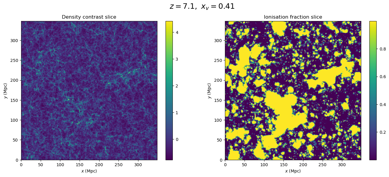
plt.suptitle('$z={0:.1f},~x_v=${1:.2f}'.format(z,xfrac.mean()), size=18)

plt.subplot(121)
plt.title('Density contrast slice')
plt.pcolormesh(x, y, dens[0]/dens.mean()-1)
plt.xlabel('$x$ (Mpc)')
plt.ylabel('$y$ (Mpc)')
plt.colorbar()

plt.subplot(122)
plt.title('Ionisation fraction slice')
plt.pcolormesh(x, y, xfrac[0])
plt.xlabel('$x$ (Mpc)')
plt.ylabel('$y$ (Mpc)')
plt.colorbar()

plt.show()

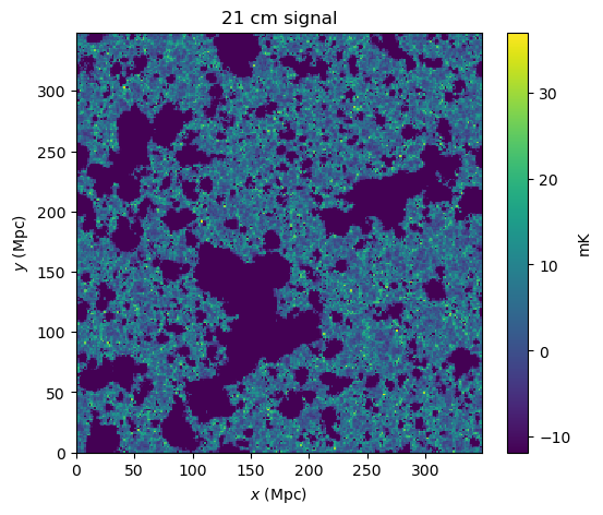
21 cm brightness temperature¶

We can construct the 21 cm brightness temperature from the density field and ionisation fraction field using calc_dt. Due to the absence of zero baseline, the mean signal will be subtracted from each frequency channel. One can use subtract_mean_signal to add this effect.

[8]:

dT = t2c.calc_dt(xfrac, dens, z)
print('Mean of first channel: {0:.4f}'.format(dT[0].mean()))

Mean of first channel: 11.8259

[9]:

dT_subtracted = t2c.subtract_mean_signal(dT, 0)
print('Mean of first channel: {0:.4f}'.format(dT_subtracted[0].mean()))

Mean of first channel: -0.0000

[10]:

plt.rcParams['figure.figsize'] = [6, 5]

plt.title('21 cm signal')
plt.pcolormesh(x, y, dT_subtracted[0,:,:])
plt.xlabel('$x$ (Mpc)')
plt.ylabel('$y$ (Mpc)')
plt.colorbar(label='mK')

plt.show()

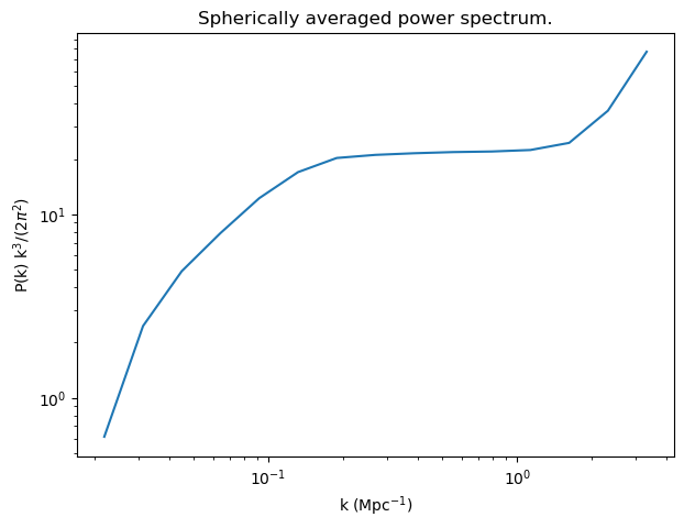
21 cm power spectrum¶

One of the most interesting metric to analyse this field is the power spectrum. Here we estimate the spherically average power spectrum using power_spectrum_1d function.

The function needs the length of the input_array in Mpc (or Mpc/h) through box_dims parameters. This is used to calculate the wavenumbers (k). The unit of the output k values will be 1/Mpc (or h/Mpc). If the input_array has unequal length in each direction, then one can provide box_dims with a list containing the lengths in each direction.

[11]:

box_dims = 244/0.7 # Length of the volume along each direction in Mpc.

[12]:

ps, ks = t2c.power_spectrum_1d(dT_subtracted, kbins=15, box_dims=box_dims)

[13]:

plt.rcParams['figure.figsize'] = [7, 5]

plt.title('Spherically averaged power spectrum.')
plt.loglog(ks, ps*ks**3/2/np.pi**2)
plt.xlabel('k (Mpc$^{-1}$)')
plt.ylabel('P(k) k$^{3}$/$(2\pi^2)$')

plt.show()

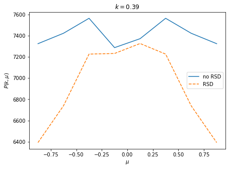
Redshift-space distortions¶

The 21 cm signal will be modified while mapping from real space to redshift space due to peculiar velocities (Mao et al. 2012).

The VelocityFile function is used to read the velocity files produced by CubeP3M. We need the velocities in km/s as a numpy array of shape (3,nGridx,nGridy,nGridyz), where the first axis represent the velocity component along x, y and z spatial direction. The get_kms_from_density attribute gives such a numpy array.

[14]:

v_file = t2c.VelocityFile(path_to_datafiles+'7.059v_all.dat')

[15]:

kms = v_file.get_kms_from_density(d_file)

The get_distorted_dt function will distort the signal.

[16]:

dT_rsd = t2c.get_distorted_dt(dT, kms, z,
                              los_axis=0,
                              velocity_axis=0,
                              num_particles=20)

Spherically averaged power spectrum of the 21 cm signal with RSD.

[17]:

ps_rsd, ks_rsd = t2c.power_spectrum_1d(dT_rsd, kbins=15, box_dims=box_dims)

[18]:

plt.rcParams['figure.figsize'] = [7, 5]

plt.title('Spherically averaged power spectrum.')
plt.loglog(ks, ps*ks**3/2/np.pi**2, label='no RSD')
plt.loglog(ks_rsd, ps_rsd*ks_rsd**3/2/np.pi**2, linestyle='--', label='RSD')

plt.xlabel('k (Mpc$^{-1}$)')
plt.ylabel('P(k) k$^{3}$/$(2\pi^2)$')
plt.legend()

plt.show()

We see in the above figure that the spherically averaged power spectrum has changed after RSD is implemented.

However, a better marker of RSD in 21 cm signal is the power spectrum’s \(\mu (\equiv k_\parallel/k)\) dependence (Jensen et al. 2013). The power spectrum of 21 cm signal with RSD will have the following dependence (Barkana & Loeb 2005),

\(P(k,\mu) = P_0 + \mu^2P_2 +\mu^4P_4\).

We can calculate \(P(k,\mu)\) using power_spectrum_mu function.

[19]:

Pk, mubins, kbins, nmode = t2c.power_spectrum_mu(
    dT,
    los_axis=0,
    mubins=8,
    kbins=15,
    box_dims=box_dims,
    exclude_zero_modes=True,
    return_n_modes=True,
    absolute_mus=False,
)

[20]:

Pk_rsd, mubins_rsd, kbins_rsd, nmode_rsd = t2c.power_spectrum_mu(
    dT_rsd,
    los_axis=0,
    mubins=8,
    kbins=15,
    box_dims=box_dims,
    exclude_zero_modes=True,
    return_n_modes=True,
    absolute_mus=False,
)

[21]:

plt.rcParams['figure.figsize'] = [7, 5]
ii = 8

plt.title('$k={0:.2f}$'.format(kbins[ii]))
plt.plot(mubins, Pk[:,ii], label='no RSD')
plt.plot(mubins_rsd, Pk_rsd[:,ii], linestyle='--', label='RSD')

plt.xlabel('$\mu$')
plt.ylabel('$P(k,\mu)$')
plt.legend()

plt.show()

Bubble size distribution¶

The bubble (HII regions) size distribution is an intersting probe of the reionization process (Giri et al. 2018).

Tools21cm contains three methods to determine the size distributions, which are Friends-of-friends, Spherical average and mean free path approach.

In this tutorial, we will take the ionisation fraction field and assume all the pixels with value \(>0.5\) as ionised.

[22]:

xHII = xfrac>0.5

boxsize = 244/0.7 # in Mpc

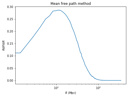
Mean free path (e.g. Mesinger & Furlanetto 2007)

[23]:

r_mfp, dn_mfp = t2c.mfp(xHII, boxsize=boxsize, iterations=1000000)

MFP method applied on 3D data (ver 1.0)
Initialising random rays...
...done
Estimating ray lengths...

 48%|███████████████████▋                     | 120/250 [00:06<00:07, 18.24it/s]

...done

Program runtime: 0.126151 minutes.
The output contains a tuple with three values: r, rdP/dr
The curve has been normalized.

[24]:

plt.rcParams['figure.figsize'] = [7, 5]

plt.semilogx(r_mfp, dn_mfp)

plt.xlabel('$R$ (Mpc)')
plt.ylabel('$R\mathrm{d}P/\mathrm{d}R$')
plt.title('Mean free path method')

plt.show()

Spherical average (e.g. Zahn et al. 2007)

[25]:

r_spa, dn_spa = t2c.spa(xHII, boxsize=boxsize, nscales=20)

100%|███████████████████████████████████████████| 20/20 [01:30<00:00,  4.51s/it]

[26]:

plt.rcParams['figure.figsize'] = [7, 5]

plt.semilogx(r_spa, dn_spa)

plt.xlabel('$R$ (Mpc)')
plt.ylabel('$R\mathrm{d}P/\mathrm{d}R$')
plt.title('Spherical Average method')
plt.show()

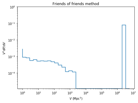
Friends of friends (e.g. Iliev et al. 2006)

[27]:

labelled_map, volumes = t2c.fof(xHII)
fof_dist = t2c.plot_fof_sizes(volumes, bins=30, boxsize=boxsize)

Program runtime: 0.015371 minutes.
The output is a tuple containing output-map and volume-list array respectively.
The output is Size, Size**2 dP/d(Size), lowest value

[28]:

plt.rcParams['figure.figsize'] = [7, 5]

plt.step(fof_dist[0], fof_dist[1])
plt.xscale('log')
plt.yscale('log')
plt.ylim(fof_dist[2],1)

plt.xlabel('$V$ (Mpc$^3$)')
plt.ylabel('$V^2\mathrm{d}P/\mathrm{d}V$')
plt.title('Friends of friends method')

plt.show()

Telescope noise calculation.¶

See Ghara et al. 2016 and Ghara et al. 2016 for more information

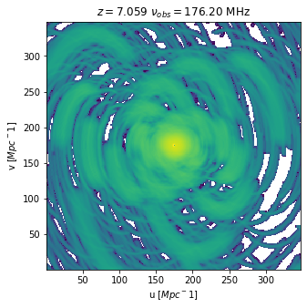
uv-coverage¶

We start with calculation of the uv-coverage for SKA1-Low configuration.

[29]:

uv, Nant = t2c.get_uv_daily_observation(ncells=dT.shape[0], # The number of cell used to make the image
                                        z=z,                # Redhsift of the slice observed
                                        filename=None,      # If None, it uses the SKA-Low 2016 configuration.
                                        total_int_time=6.0, # Observation per day in hours.
                                        int_time=10.0,      # Time period of recording the data in seconds.
                                        boxsize=boxsize,    # Comoving size of the sky observed
                                        declination=-30.0,
                                        verbose=True)

Making uv map from daily observations.

100%|███████████████████████████████████████| 2159/2159 [04:09<00:00,  8.65it/s]

...done

We suggest that you save the uv map as it is computationally expensive. Expecially when computed for an array of redshifts.

[30]:

np.save(path_to_datafiles+'uv_map.npy', uv)
np.save(path_to_datafiles+'Nant.npy', Nant)

[31]:

plt.rcParams['figure.figsize'] = [5, 5]

plt.title(r'$z=%.3f$ $\nu_{obs}=%.2f$ MHz' %(z, t2c.z_to_nu(z)))
plt.pcolormesh(x, y, np.log10(np.fft.fftshift(uv)))
plt.xlabel('u [$Mpc^-1$]'), plt.ylabel('v [$Mpc^-1$]');

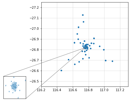
Here we plot the antennas location of the SKA1-Low configuration.

[32]:

from mpl_toolkits.axes_grid1.inset_locator import inset_axes
from mpl_toolkits.axes_grid1.inset_locator import mark_inset

ska_ant = t2c.SKA1_LowConfig_Sept2016()

fig, ax = plt.subplots(figsize=(5, 5))
plt.plot(ska_ant[:,0], ska_ant[:,1], '.')
x1, x2, y1, y2 = 116.2, 117.3, -26.45, -27.25
ax.set_xlim(x1, x2)
ax.set_ylim(y1, y2)
ax.grid(b=True, alpha=0.5)

axins = inset_axes(ax, 1, 1, loc=4, bbox_to_anchor=(0.2, 0.2))
plt.plot(ska_ant[:,0], ska_ant[:,1], ',')
x1, x2, y1, y2 = 116.75, 116.78, -26.815, -26.833
axins.set_xlim(x1, x2)
axins.set_ylim(y1, y2)
axins.grid(b=True, alpha=0.5)
mark_inset(ax, axins, loc1=4, loc2=2, fc="none", ec="0.5")
axins.axes.xaxis.set_ticks([]);
axins.axes.yaxis.set_ticks([]);

Creating the noise cube¶

[33]:

noise_cube = t2c.noise_cube_coeval(ncells=dT.shape[0],
                                   z=z,
                                   depth_mhz=None,   #If None, estimates the value such that the final output is a cube.
                                   obs_time=1000,
                                   filename=None,
                                   boxsize=boxsize,
                                   total_int_time=6.0,
                                   int_time=10.0,
                                   declination=-30.0,
                                   uv_map=uv,
                                   N_ant=Nant,
                                   verbose=True,
                                   fft_wrap=False)

Creating the noise cube...

100%|████████████████████████████████████████| 250/250 [00:02<00:00, 120.25it/s]

[34]:

plt.rcParams['figure.figsize'] = [16, 6]

plt.suptitle('$z=%.3f$ $x_v=%.3f$' %(z, xfrac.mean()), size=18)
plt.subplot(121)
plt.title('noise cube slice')
plt.pcolormesh(x, y, noise_cube[0])
plt.colorbar(label='$\delta T^{noise}$ [mK]')
plt.subplot(122)
plt.title('noise distribution')
plt.hist(noise_cube.flatten(), bins=150, histtype='step');
plt.xlabel('$\delta T^{noise}$ [mK]'), plt.ylabel('$N_{sample}$');

Create realistic 21-cm observational images¶

To create realistict observational images we combined the 21-cm filed with the noise cube and smooth the data to the resolution corresponding to maximum baseline of 2 km. The smoothing works for any kind of data (e.g. xHII, dT, etc.) and also for single dish. In the former case the max_baseline should be substituted to D/122, where D is the antenna disk diameter.

[35]:

dT2 = dT_subtracted + noise_cube

dT_smooth = t2c.smooth_coeval(cube=dT2,    # Data cube that is to be smoothed
                              z=z,                  # Redshift of the coeval cube
                              box_size_mpc=boxsize, # Box size in cMpc
                              max_baseline=2.0,     # Maximum baseline of the telescope
                              ratio=1.0,            # Ratio of smoothing scale in frequency direction
                              nu_axis=2)            # frequency axis

100%|████████████████████████████████████████| 250/250 [00:00<00:00, 268.96it/s]

[36]:

plt.rcParams['figure.figsize'] = [15, 6]

plt.subplot(121)
plt.title('$\delta T_b$ at simulation resolution')
plt.pcolormesh(x, y, dT[0])
plt.colorbar(label='$\delta T_b$ [mK]')
plt.subplot(122)
plt.title('smoothed $\delta T_b + \delta T^{noise}_b$')
plt.pcolormesh(x, y, dT_smooth[0])
plt.colorbar(label='$\delta T_b$ [mK]')

[36]:

<matplotlib.colorbar.Colorbar at 0x7efefecf6370>

Image segmenation with Tools21cm¶

The Identification of HII regions in noisy 21-cm interferometric images is not trivial. Tools21cm contains two methods to identify (segmentation) ionised/neutral regions: the super-pixel method Giri et al. 2018 and the deep learning algorithm SegU-Net Bianco et al. 2022.

In this tutorial, we will take the ionisation fraction field and assume all the pixels with value \(>0.5\) as ionised.

The superpixel algorithm¶

We start by calculating the superpixel labels

[37]:

%%time
labels = t2c.slic_cube(cube=dT_smooth,
                       n_segments=5000,
                       compactness=0.1,
                       max_iter=20,
                       sigma=0,
                       min_size_factor=0.5,
                       max_size_factor=3,
                       cmap=None)

Estimating superpixel labels using SLIC...
The output contains the labels with 4911 segments
CPU times: user 3min 42s, sys: 375 ms, total: 3min 42s
Wall time: 3min 43s

Make the superpixel cube and plot a slice.

[38]:

superpixel_map = t2c.superpixel_map(dT_smooth, labels)

plt.rcParams['figure.figsize'] = [18, 5]
plt.subplot(131)
plt.pcolormesh(x, y, superpixel_map[0], cmap='jet')
plt.subplot(132)
plt.pcolormesh(x, y, dT_smooth[0], cmap='jet')

Estimating the superpixel mean map...

100%|████████████████████████████████████| 4911/4911 [00:00<00:00, 51612.08it/s]

...done
Constructing the superpixel map...

100%|███████████████████████████████████████| 4911/4911 [01:16<00:00, 64.19it/s]

[38]:

<matplotlib.collections.QuadMesh at 0x7efefecf3b50>

Stitch the superpixels using the superpixel PDFs and plot a slice from identified ionized region cube. Then smooth the true ionisation fraction field to compare.

[39]:

xHII_stitch = t2c.stitch_superpixels(data=dT_smooth,
                                     labels=labels,
                                     bins='knuth',
                                     binary=True,
                                     on_superpixel_map=True)

mask_xHI = t2c.smooth_coeval(xfrac, z, box_size_mpc=boxsize, max_baseline=2.0, nu_axis=2) < 0.5

Estimating the superpixel mean map...

100%|████████████████████████████████████| 4911/4911 [00:00<00:00, 57067.18it/s]

...done
Constructing the superpixel map...

100%|███████████████████████████████████████| 4911/4911 [01:21<00:00, 60.60it/s]
100%|████████████████████████████████████████| 250/250 [00:01<00:00, 194.97it/s]

[40]:

from sklearn.metrics import matthews_corrcoef

phicoef_sup = matthews_corrcoef(mask_xHI.flatten(), 1-xHII_stitch.flatten())

plt.rcParams['figure.figsize'] = [12, 6]
plt.subplot(121)
plt.title('Super-Pixel: $r_{\phi}=%.3f$' %phicoef_sup)
plt.pcolormesh(x, y, 1-xHII_stitch[0], cmap='jet')
plt.contour(mask_xHI[0], colors='lime', extent=[0, boxsize, 0, boxsize])

[40]:

<matplotlib.contour.QuadContourSet at 0x7eff00837ee0>

SegU-Net¶

Here, we load the best performing network and calculate the nubmer of manipulation on the cube to evaluate the pixel-uncertainty. Additionally, we can get pixel-error maps

tta = 0 : super-fast (approximatelly 7 sec), it tends to be a few percent less accurate (within 2% differences), no pixel-error map (no TTA manipulation)
tta = 1 : fast (about 17 sec), accurate, with pixel-error map (3 samples)
tta = 2 : slow (about 10 min), accurate, with pixel-error map (~100 samples)

[42]:

seg = t2c.segmentation.segunet21cm(tta=2, verbose=True)

tot number of (unique) manipulation we can do on a cube: 28
 Loaded model: /home/michele/codes/tools21cm/src/tools21cm/input_data/segunet_03-11T12-02-05_128slice_ep35.h5

In the current version of Tools21cm, the network operates on data cubes with a mesh size of \(128^3\). In future updates, we plan to extend to cover the mesh size of any given input. Moreover, SegU-Net is optimised for cube data with and spatial resolution of \(2\,Mpc\). However, it deals well with simulation with smaller resolution.

For the reason mentioned above, here we cut the differential brightness cube and Super-Pixel output in order to match SegU-Net input shape.

[43]:

dT_cut = dT_smooth[:128,:128,:128]
mask_xHI2 = mask_xHI[:128,:128,:128]

xHI_seg, xHI_seg_err = seg.prediction(x=dT_cut)
phicoef_seg = matthews_corrcoef(mask_xHI2.flatten(), xHI_seg.flatten())

xHI_sup = xHII_stitch[:128,:128,:128]
phicoef_sup = matthews_corrcoef(mask_xHI2.flatten(), 1-xHI_sup.flatten())

100%|███████████████████████████████████████████| 28/28 [19:38<00:00, 42.09s/it]

[46]:

fig, axs = plt.subplots(figsize=(12,6), ncols=3, sharey=True, sharex=True)
(ax0, ax1, ax2) = axs

ax0.set_title('Super-Pixel ($r_{\phi}=%.3f$)' %phicoef_sup)
ax0.imshow(1-xHI_sup[0], origin='lower', cmap='jet', extent=[0, boxsize, 0, boxsize])
ax0.contour(mask_xHI2[0], colors='lime', extent=[0, boxsize, 0, boxsize])
ax0.set_xlabel('x [Mpc]')

ax1.set_title('SegU-Net ($r_{\phi}=%.3f$)' %phicoef_seg)
ax1.imshow(xHI_seg[0], origin='lower', cmap='jet', extent=[0, boxsize, 0, boxsize])
ax1.contour(mask_xHI2[0], colors='lime', extent=[0, boxsize, 0, boxsize])
ax1.set_xlabel('x [Mpc]')

ax2.set_title('SegUNet Pixel-Error')
im = ax2.imshow(xHI_seg_err[0], origin='lower', cmap='jet', extent=[0, boxsize, 0, boxsize])
fig.colorbar(im, label=r'$\sigma_{std}$', ax=ax2, pad=0.02, cax=fig.add_axes([0.905, 0.25, 0.02, 0.51]))
ax2.set_xlabel('x [Mpc]')

plt.subplots_adjust(hspace=0.1, wspace=0.01)
for ax in axs.flat: ax.label_outer()